[논문] Attention Is All You Need (2017)

논문/AI

[논문] Attention Is All You Need (2017)

guungyul 2024. 12. 29. 13:24

Attention Is All You Need

The dominant sequence transduction models are based on complex recurrent or convolutional neural networks in an encoder-decoder configuration. The best performing models also connect the encoder and decoder through an attention mechanism. We propose a new

arxiv.org

연속적인 sequence input을 처리하는 기존 모델들은 CNN이나 RNN 등 복잡한 nerual network 구조에 encoder와 decoder를 사용합니다. 본 논문에서는 기존 복잡한 구조를 벗어나 attention mechanism 만을 사용한 간단한 Transformer 모델을 소개합니다.

1 Introduction

Sequence modeling과 transduction의 기존 state of the art 모델들

Recurrent neurla networks, long short-term memory, gated recurrent neural networks
- Input과 output sequence에서 symbol의 위치를 반영한 계산
- Sequential한 계산 때문에 parallelization을 할 수 없음
  - 따라서 sequence 길이가 길어질수록 memory contraint

Attention mechanism은 input과 output sequence의 거리에 상관없이 두 symbol의 의존 관계를 모델링 할 수 있다.

본 논문에서는 attention mechanism만을 사용해 input과 output의 전역적인 의존 관계를 얻는 Transformer 모델 구조를 제시한다.

2 Background

Self-attention

입력 sequence 안의 다양한 위치간 관계를 학습하여 해당 sequence의 표현을 계산하는 attention 기법

Transformer는 RNN이나 CNN 없이 self-attention만을 사용해 input과 output sequence의 표현을 계산하는 첫번째 모델이다.

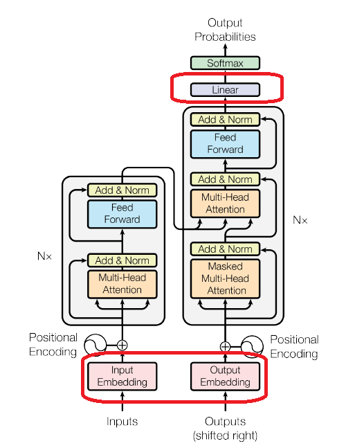
3 Model Architecture

Encoder-decoder sturcture

Encoder는 input sequence $ (x_1, ..., x_n) $를 연속적인 표현 $ z = (z_1, ..., z_n) $으로 나타냄
Decoder는 z를 활용해 output sequence $ (y_1, ..., y_m) $ symbol을 하나씩 생성

각 단계에서 모델은 auto-regressive 하다.

이전에 생성된 symbol을 다음 symbol을 생성할 때 추가적인 input으로 사용

Transformer는 encoder와 decoder에 모두 stacked self-attention과 독립적 연산을 수행하는 fully-connected layer를 가진다.

3.1 Encoder and Decoder Stacks

Encoder

총 6개의 동일한 layer가 stack 되어 있음
각 layer는 두개의 sub-layer로 구성
- Multi-head self-attention 기법
- Simple, position-wise fully connected feed-forward network
각 sub-layer에는 residual connection과 정규화가 적용됨
- Residual connection: 입력 데이터를 출력에 더하는 연결 방식
- Sub-layer output: $ LayerNorm(x + Sublayer(x)) $
모든 sub-layer와 embedding layer에서의 output dimension은 512
- $ d_{model} = 512 $

Decoder

총 6개의 동일한 layer가 stack 되어 있음
Encoder에 있는 두개의 sub-layer 외에 추가로 세번째 sub-layer를 가짐
- Encoder의 output에 multi-head attention 을 수행하는 sub-layer
  - Figure 1 그림 오른쪽 중간 sub-layer
Encoder와 동일하게 각 sub-layer에는 residual connection과 정규화가 적용됨
Self-attention sub-layer가 나중에 오는 위치를 참고하지 않게 masking 진행
- Position $ i $의 예측값은 position $ i $ 보다 작은 위치 값 output에만 영향을 받음
  - Figure 1 그림 오른쪽 가장 밑 sub-layer

3.2 Attention

Attention
- Query와 key-value pair를 output으로 mapping
  - Output은 query와 key로 계산되는 weight를 사용한 weighted sum으로 계산됨
  - Query, keys, values는 모두 vector
- 예시
  - 문장: I have a dog named Toto.
  - Q (질문): Toto (연관성을 구하고자 하는 단어)
  - K (가능한 정답): [I, have, a, dog, named, Toto] (모든 문장 단어)
  - V (의미가 담긴 embedding): 각 단어의 embedding
    - $ Weight = f(Q, K)) $
    - $ Output = Weight * V $

3.2.1 Scaled Dot-Product Attention

Input

Queries and keys with dimension $ d_k $
Values with dimension $ d_v $

실제로 여러 query들을 동시에 matrix 형태로 계산

$$ \text{Attention}(Q, K, V) = \text{softmax}\left(\frac{QK^T}{\sqrt{d_k}}\right)V $$

두가지 attention 함수가 존재

Additive attention
Dot-product attention
- Dot-product가 더 빠르고 space-efficient
- $d_k$ 값이 커질수록 dot-product 기법이 더 느려짐
  - 따라서 scale factor $ \frac{1}{\sqrt{d_k}} $를 추가

3.2.2 Multi-Head Attention

$ d_{model}로 하나의 attention function을 수행하는 것 보다 효과적인 방법을 사용: Multi-head attention

Query, keys, values를 각각 학습된 linear projection으로 h번 $d_k, d_k, d_v$ dimension으로 project
Project 된 queries, keys, values에 attention function을 병렬적으로 수행
- 이때 $ d_k = \frac{d_{model}}{num of heads} $
- $ d_v $ dimension output 도출
- Output들은 다시 합치고 project 해서 최종 values를 도출

Multi-head attention은 모델이 서로 다른 representation subspace에서의 정보를 서로 다른 위치에서 참조할 수 있도록 한다.

Representation subspace로 다양한 표현을 embedding

예시: Semantic meaning, grammatical structure, part-of-speech 등
Single-head attention에서는 불가능

3.2.3 Aplications of Attention in our Model

Transformer는 multi-head attention을 세가지 다른 방법으로 사용:

"Encoder-decoder attention" layer
- Queries는 이전 decoder layer로부터 옴
- Keys와 values는 encoder의 output으로 부터 옴
- Decoder의 모든 위치에서 input sequence의 모든 위치를 참조할 수 있게 함
  - 이는 sequence-to-sequence 모델의 encoder-decoder attention 기법을 모방
- Encoder의 input sequence와 decoder의 output sequence 사이에 연관성을 학습
Self-attention layers in encoder
- 모든 keys, values, queries는 이전 encoder layer로 부터 옴
- Encoder의 모든 위치에서 이전 encoder layer의 모든 위치를 참조할 수 있게 함
- Input sequence의 각 위치에 대한 연관성을 학습
Self-attention layers in decoder
- 비슷하게 decoder의 모든 위치에서 현재 위치까지의 모든 위치를 참조할 수 있게 함
- Auto-regressive하도록 masking을 진행
  - Sclaed dot-product attention에서 future token softmax input을 $ -\infty $로 mask
- Output sequence의 각 위치에 대한 연관성을 학습

3.3 Position-wise Feed-Forward Networks

Fully connected feed-forward network

각 위치에 동일하게 적용
Linear transformation -> ReLU activation -> Linear transformation

$$ \text{FFN}(x) = \max(0, xW_1 + b_1)W_2 + b_2 $$

각 위치에 동일한 linear transformation이 적용
각 layer 마다 다른 parameter를 사용
$d_{model} = 512 $
$d_{ff} = 2048 $

3.4 Embeddings and Softmax

Learned embedding을 사용해 input token과 output token을 $ d_{model} $로 변환
Learned linear transforamtion와 softmax 함수를 사용해 decoder output으로 다음 토큰 확률을 계산
두 embedding layer와 pre-softmax linear transformation에 같은 weight matrix를 사용
- Embedding layer에서는 weight를 $ \sqrt{d_{\text{model}}} $로 곱함

3.5 Positional Encoding

토큰의 위치 정보를 추가하기 위해 정보를 주입해야 한다.

Input embedding에 positional encoding을 추가
- Dimension: $ d_{model} $

$$ PE_{\text{(pos, 2i)}} = \sin\left(\frac{\text{pos}}{10000^{2i/d_{\text{model}}}}\right) $$
$$ PE_{\text{(pos, 2i+1)}} = \cos\left(\frac{\text{pos}}{10000^{2i/d_{\text{model}}}}\right) $$

pos: 위치
i: dimension
Sinusoid 함수 모양을 가짐

다른 positional embedding 기법을 사용해도 거의 유사한 결과를 얻음

4 Why Self-Attention

기존 RNN과 CNN에 비해 self-attention이 가지는 장점

더 낮은 계산 복잡도
병렬화 될 수 있는 계산 양
네트워크내 long-range dependencies의 path 길이
해석 가능한 모델

5 Training

5.1 Training Data and Batching

WMT 2014 English-German dataset

4.5 million sentence paris
Byte-pair encoding 사용
- source-target 어휘 약 37000 tokens

WMT 2014 English-French dataset

36M sentence paris
32000 word-piece 어휘로 분리

각 training batch는 25000 source tokens과 25000 target token을 가지는 문장 pair로 구성

5.2 Hardware and Schedule

8 NVIDIA P100 GPUs

Base model: 100,000 steps

Big model: 300,000 steps

5.3 Optimizer

Adam optimizer

$ \beta_1 = 0.9, \, \beta_2 = 0.98, \, \epsilon = 10^{-9} $

Learning rate

$$ \text{lrate} = d_{\text{model}}^{-0.5} \cdot \min\left(\text{step}_{num}^{-0.5}, \text{step}_{num} \cdot \text{warmup}_{steps}^{-1.5}\right) $$

$ warmup_steps = 4000 $

5.4 Regularization

Residual Dropout
- 모든 sub-layer output에 적용
- $ P_{drop} = 0.1 $
Label Smoothing
- $ \epsilon_{ls} = 0.1 $

6 Results

6.1 Machine Translation

WMT 2014 English-to-German: Big transformer 모델이 기존 모델들보다 더 좋은 성능을 보임
WMT 2014 English-to-French: Big transformer 모델이 기존 모델들보다 더 좋은 성능을 보임
- $ P_{drop} $을 0.3이 아닌 0.1을 사용
Base model: Average 5 checkpoints
Big model: Average 20 checkpoints
Beam search
- Size 4
- Length penalty $ \alpha = 0.6 $

6.2 Model Variations

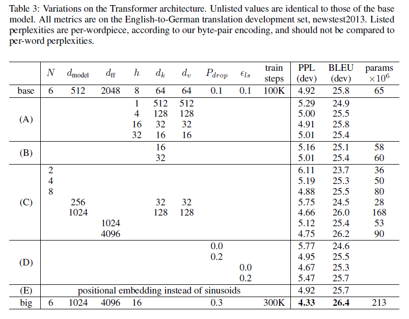
Base model에 변화를 줘 newstest2013 English-to-German 번역에서의 성능을 테스트 한 결과이다.

같은 bean search 방법을 사용하고 checkpoint averaging은 사용하지 않았다.

Row A
- Attention heads 개수와 attention key, value 차원에 변화를 줌
- Head 수가 1개일 때 또 head 수가 너무 많을 때 성능이 저하됨
Row B
- Attention key 사이즈를 줄임
- 성능이 저하됨
- 단순한 dot-product가 아닌 다른 방법이 효과적일 수 있음
Row C & Row D
- 더 큰 모델 성능이 더 좋음
- Dropout은 over-fitting을 피하는데 아주 효과적임
Row E
- Sinusoidal positional encoding을 learned positional embedding으로 바꿈
- 거의 똑같은 결과를 얻음

6.3 English Constituency Parsing

모델 일반화를 테스트하기 위해 English constituency parsing을 진행한다

문장을 구성 성분으로 나누고 계층적 구조를 파악하는 작업

Model

4-layer transformer with $ d_{model} = 1024 $
Beam size 21, $ \alpha = 0.3 $
다른 hyperparameter는 English-to-German 번역 모델과 동일

Dataset

Wall Street Journal 40K sentences
- 16K token 사용
BerkleyParser corpora 17M sentences in semi-supervised
- 32K token 사용

Result

Recurrent Neural Network Grammar 외에 다른 모든 모델보다 더 좋은 성능을 보여줌

7 Conclusion

본 논문에서는 attention 기법만을 사용한 sequence transduction 모델을 소개한다.

WMT 2014 English-to-German 과 WMT 2014 English-to-French 번역 작업에서 모두 기존 모델들보다 좋은 성능을 보여준다.

GitHub link: https://github.com/tensorflow/tensor2tensor